Analysis of Kinase-based Viral Drug Connectivity Mapping
Intro
Kinases are pretty exciting to me, not only because protein phosphorylation plays a role in regulating most aspects of cell life, but also because abnormal phosphorylation is often the cause or consequence of disease. Accordingly, they've become an important group of drug targets that I wanted to take a look at.
In an attempt to unearth some computational biology skills, review some recent Pandas exposure, and get back into the spirit of biological research and discovery, I wanted to explore the relationship between kinase differential expression and viral infection. To do so, I ran a general query on the Gene Expression Atlas for all experiments that had to deal with viruses and for genes somehow related to kinases. Following this, the ultimate goal was to use connectivity mapping to find possible drug candidates correlated with a reversion in differential expression.
Some Background + Motivation
Recently, one of five 2016 Breakthrough Prizes in the Life Sciences was awarded to Professor Stephen Elledge, who among other incredible things is particularly known for his work in eludicating the human DNA damage response. Excitingly, this can basically be summarized as a protein kinase cascade, and so one could imagine directing their drug discovery search in regards to diseases that heavily involve DNA damage towards kinase inhibitors or activators. Cancers are probably what come to mind the most, and I had also done some Pandas notebook exploration into that, but many cells also undergo virus infection-associated DDR.
Picking the right virus infection targets
Another motivating idea is that going after viruses is difficult, particularly because of their rapid mutation cycle frequently rendering drugs obsolete. While we typically think of targeting foreign proteins such as external envelope proteins, another path to take might involve looking elsewhere from the virus entirely, and instead at host targets. While this sounds kind of like targeting your own cells with a therapeutic meant to kill viruses, viral infection might cause the upregulation of certain genes in host cells that allow them to propogate. If we can disrupt these then, the virus has a much harder time of getting by, and can't quite rely on its typical mutation frequency to escape dependency as fast. The idea is that drugs that disrupt host pathways that the virus relies on can't be as easily overcome by the virus through mutation because that would require the virus to evolve an entirely different functionality, which is a much lower probability event then changing a few coat protein residues.
More motivation
Along with talking to Dr. Andrew Taube at DESRES and learning about their group's work in MD with kinases, phosphatases, and viruses, and having my own probably farfetched ideas about one day being able to engineer a sort of hyper DDR and immunity against the introduction of viral DNA, I was interested in seeing what I could find through a short exploration with publically available datasets and Pandas tools.
I had also just taken MCB60: Cellular Biology and Molecular Medicine, which involved a lab component exploring DDR in yeast (slides viewable here). Three months of intermittent web lab work is kind of naturally inconclusive, so I was eager to see if I could get some more definite results computationally.
While in the short time putting this together I could only get as far as generating possibly connected drugs that would work towards reversing host cell expression after virus infection, and there's still a ton of analysis to be done with more time, the exercise was pretty fun and interesting. The later parts of the notebook could also definitely be cleaned up.
%matplotlib inline

import pandas as pd
import matplotlib.pyplot as plt
Load data of all virus experiments with differential expression of kinase-associated genes
df_diff_exp = pd.read_table('differentialResults-kinaseAndVirus.tsv')
df_diff_exp_up = df_diff_exp.loc[df_diff_exp['log2foldchange'] >= 0]
df_diff_exp_down = df_diff_exp.loc[df_diff_exp['log2foldchange'] < 0]
View all experiments
df_diff_exp['Comparison'].drop_duplicates().head()
Isolating one experiment
As a first workthrough example, we'll look at the 'PR8 influenza virus' vs 'none' in 'wild type' experiment and assign the data to the df_diff_exp_0 dataframe.
df_diff_exp_0 = df_diff_exp.loc[df_diff_exp['Comparison']==df_diff_exp['Comparison'][0]]
df_diff_exp_0.head()
Separating genes into up and down regulation dataframes
df_diff_exp_0_up = df_diff_exp_0.loc[df_diff_exp_0['log2foldchange'] > 0]
df_diff_exp_0_down = df_diff_exp_0.loc[df_diff_exp_0['log2foldchange'] < 0]

df_diff_exp_0_up['Experiment Accession'] = df_diff_exp_0['Experiment Accession']
df_diff_exp_0_down['Experiment Accession'] = df_diff_exp_0['Experiment Accession']
Connecting to Biomart
Connects to a pretty versatile server for annotating and querying for various components (CMAP tags, Ensembl gene names, etc.)
Install module, define function to retrieve and query database
from biomart import BiomartServer
bm_server = BiomartServer('http://www.ensembl.org/biomart')
# bm_server.show_datasets()

# Use the GRCh38.p7 human ensemble dataset
hs_ensembl = bm_server.datasets['hsapiens_gene_ensembl']
Defining a get_probeset function
Returns dataframe with Ensembl Gene ID and Affy HG U133A probeset from the Biomart Ensembl server
- Requires a dataframe with a
Genecolumn name specifying the Ensembl code, and the Biomart Ensembl server previously specified.
def get_probeset(df, server):
    response = server.search({
            'filters': {
                'with_affy_hg_u133a': True,
                'ensembl_gene_id': df['Gene'].tolist()
            },
            'attributes': [
                'ensembl_gene_id', 'affy_hg_u133a'
            ]
        })
    try:
        df_probeset = pd.DataFrame([line.decode('utf-8').split('\t') for line in response.iter_lines()],
                                   columns=['Gene ID', 'Affy HG U133A probeset'])
        df_probeset['Experiment Accession'] = df['Experiment Accession']
        return df_probeset
    except:
        # Inserts placeholder gene (involved in red-green color blindness) if gene set is empty
        df_empty_probeset = pd.DataFrame({'Gene ID': ['ENSG00000102076'], 'Affy HG U133A probeset': ['221327_s_at']})
        df_empty_probeset['Experiment Accession'] = df['Experiment Accession']
        print('Empty dataset encountered. 0 probes returned')
        return df_empty_probeset
Getting probe sets for first experiment
df_probeset_0_up = get_probeset(df_diff_exp_0_up, hs_ensembl)
df_probeset_0_down = get_probeset(df_diff_exp_0_down, hs_ensembl)
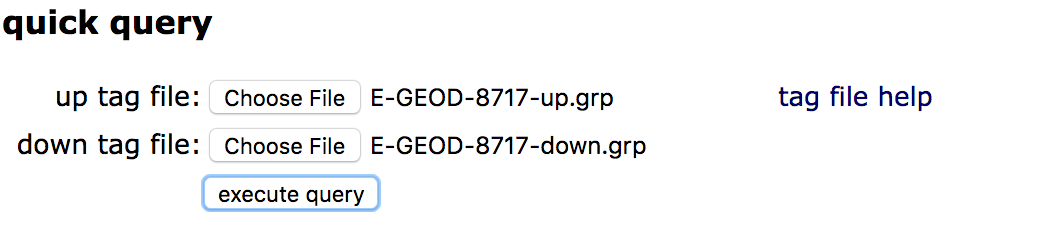
Convert to .grp files for CMap querying
The Broad Institute Connectivity Map generates gene expression signatures associated with perturbations by certain small molecule drugs.
To query the service, the project builds signatures based on lists of HG-U133A probe sets associated with the up- and down-regulated genes stored in .grp files.
Function to do all of the above
Generates .grp files ready for CMap querying
*Note: make sure to have a directory named whatever you specify the dirname parameter in the same path level as the notebook directory
def save_cmap_tags(df, server, filename, dirname, lim=0):
    df_probeset = get_probeset(df, server)
    if lim > 0:
        df_probeset = df_probeset[:lim]
    numtags = df_probeset.shape[0]
    if numtags > 200:
        print('Recommended to limit max number of tags to 200')
    df_probeset['Affy HG U133A probeset'].drop_duplicates().to_csv(path=str(dirname)+'/'+str(filename)+'.grp', sep='\t', index=None)
save_cmap_tags(df_diff_exp_0_up, hs_ensembl, 'probesets_exp_0_up', 'probesets')
save_cmap_tags(df_diff_exp_0_down, hs_ensembl, 'probesets_exp_0_down', 'probesets')
Function to generate CMap query tags from Gene Expression Atlas upload
i.e. doing almost all of the above in one method for all experiments
Because automation is good.
Possibly helper functions are noted below. (Example follows afterward).
*Note: make sure to have a directory named whatever you specify the dirname parameter in the same path level as the notebook directory
def save_cmap_tags_from_atlas(df, reg, server, dirname, lim=0):
    if reg == 0:
        diff_id = '-down'
    elif reg == 1:
        diff_id = '-up'
    df.groupby('Experiment Accession') \
        .apply(lambda df: save_cmap_tags(split_diff_exp(df, reg), server, str(df['Experiment Accession'] \
                                                                              .iloc[0])+diff_id, dirname))
Function to isolate experiment by Experiment Accession
def get_single_diff_exp(df, access_id):
    df_single_diff_exp = df.loc[df['Experiment Accession'] == access_id]
    return df_single_diff_exp
get_single_diff_exp(df_diff_exp, 'E-GEOD-13637').head(2)
Function to isolate data into up- and down-regulated gene sets
Parameter reg should be an integer 0 or 1
- 0 denotes downregulated genes
- 1 denotes upregulated genes
def split_diff_exp(df, reg):
    if reg == 0:
        return df.loc[df['log2foldchange'] < 0]
    elif reg == 1:
        return df.loc[df['log2foldchange'] > 0]
# Example building on above. Note the return of all positive log2 fold changes
split_diff_exp(get_single_diff_exp(df_diff_exp, 'E-GEOD-13637'), 1).sort_values('log2foldchange', ascending=True).head()
Saving CMap tags
# Hacky way to get both down- and up-regulated tag probe sets
for i in range(0, 2):
    save_cmap_tags_from_atlas(df=df_diff_exp, reg=i, server=hs_ensembl, dirname='probesets')
The result:
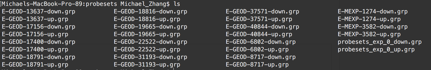
*Note: last 2 files are artifacts of the example workthrough.
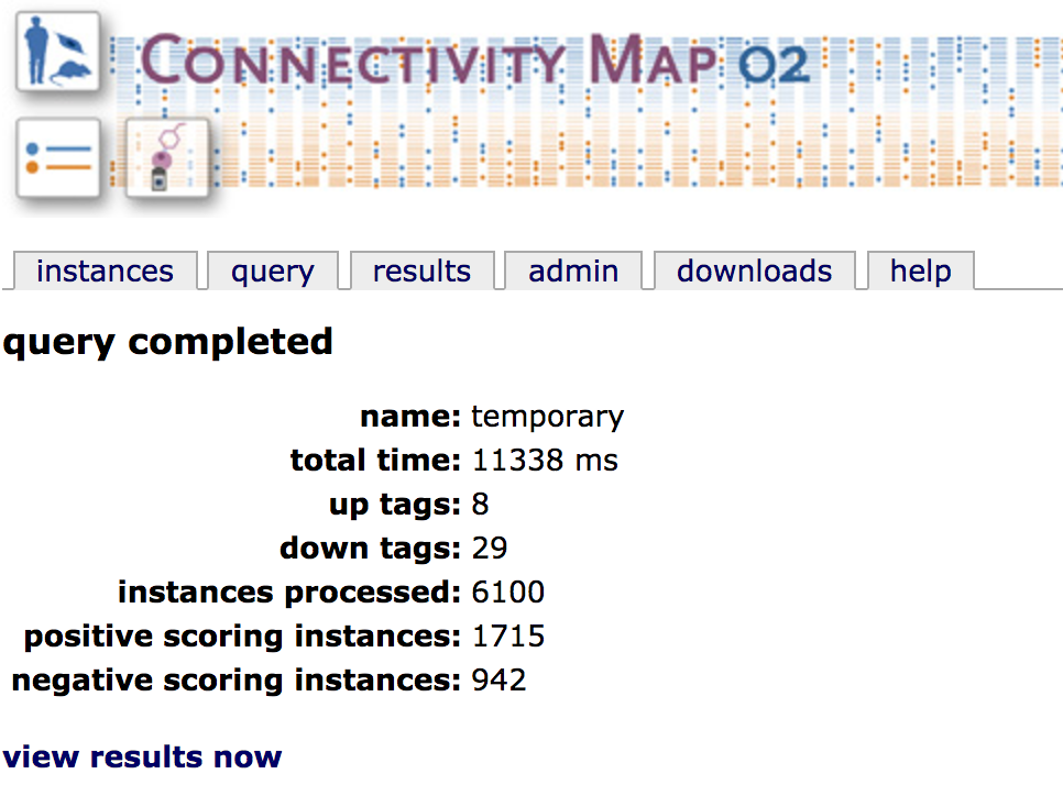
Analysis of connectivity with CMAP
We now have .grp probe set files that can be used to generate a signature and query for CMAP. After doing so, we can download the resulting table to identify perturbations that have antagonistic gene expression effects denoted by negative enrichment scores (which could be good for identifying possible drugs).
df_E_GEOD_8717 = pd.read_excel('permutedResults-E-GEOD-8717.xls')
df_E_GEOD_8717.head()
Identifying possible connected drug candidates
def find_candidates(df):
    df_cand = df.loc[df['enrichment'] < 0].sort_values(['rank', 'enrichment'], ascending=True)
    return df_cand

find_candidates(df_E_GEOD_8717).head()
Loading all CMap dataframes
df_E_GEOD_13637 = pd.read_excel('permutedResults-E-GEOD-13637.xls')
df_E_GEOD_17156 = pd.read_excel('permutedResults-E-GEOD-17156.xls')
df_E_GEOD_17400 = pd.read_excel('permutedResults-E-GEOD-17400.xls')
df_E_GEOD_18791 = pd.read_excel('permutedResults-E-GEOD-18791.xls')
df_E_GEOD_18816 = pd.read_excel('permutedResults-E-GEOD-18816.xls')
df_E_GEOD_19665 = pd.read_excel('permutedResults-E-GEOD-19665.xls')
df_E_GEOD_22522 = pd.read_excel('permutedResults-E-GEOD-22522.xls')
df_E_GEOD_31193 = pd.read_excel('permutedResults-E-GEOD-31193.xls')
df_E_GEOD_37571 = pd.read_excel('permutedResults-E-GEOD-37571.xls')
df_E_GEOD_40844 = pd.read_excel('permutedResults-E-GEOD-40844.xls')
df_E_MEXP_1274 = pd.read_excel('permutedResults-E-MEXP-1274.xls')
df_E_MEXP_3582 = pd.read_excel('permutedResults-E-MEXP-3582.xls')
find_candidates(df_E_GEOD_13637)[:100]
Future Analysis To Go Here